Approximate your spending pattern using Gradient descent in FSharp
Approximate your spending pattern using Gradient descent in FSharp
The advantage of tracking your expenses is that you can compare each month and check if you saved more or less money than the previous month. Another interesting information is to know how fast you are spending your money. Checking how fast you spend your money gives you a hint on whether you are likely to be out or within budget at the end of the month.
The easiest way to check that is to plot the daily cumulated sum of your expenses and compare each month. I have been doing this for the past few months and it worked pretty well but I realised that the cumulated sum is not always nice to look at. It looks like incremental steps which is not so pleasing to the eye. As soon as you have more than three cumulated sum plotted on the same graph, it becomes messy and hard to see.
The goal is to be able to be able to understand your financial situation in a glance, without having to spend more than one second a the plot.
This is were having straight lines can be more practical. Straight lines are much more pleasing to the eye than incremental steps so it would be much nicer if I could transform supermarket expenses montly curves to straight lines but how do I transform points to a straight line?
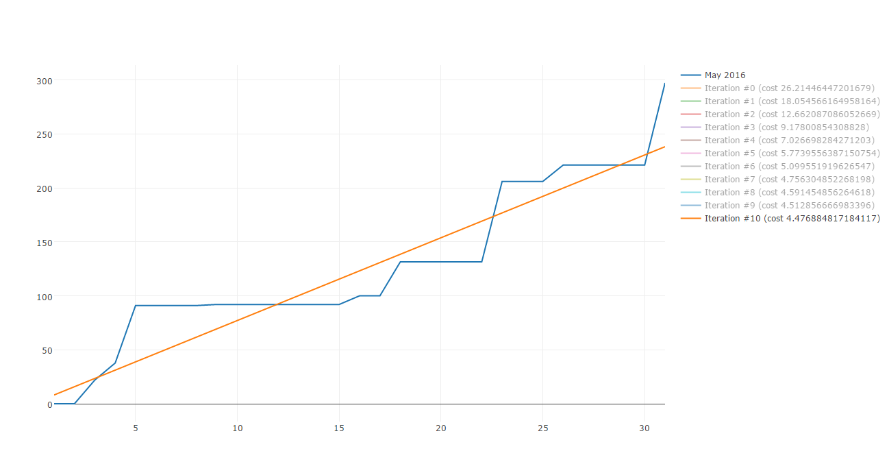
Lucky me there are plenty of algorithms to build straight line approximations. Gradient descent is one of those. Here is a sample of Gradient descent iterations:
Today I would like to share how you can use Gradient descent to approximate your spending patterns. This post is composed by three parts:
- Why approximate to a straight line and what is Gradient descent
- Cost function and algorithm
- Apply to real life data with F#
1. Why approximate to a straight line and what is Gradient descent
As you see from the plot in the introduction, real life data like supermarket expenses aren’t consistant. Therefore it is hard to make any estimation apart from visual estimation. What we want is to reduce that function to the most simplistic function without having to much error. If we manage to reduce the curve to a first degree equation (straight line), we will be able to approximate on each day how much the expenses will be. Therefore using this approximation can help us, when we are in the middle of the month, to approximate the rest of the month and check whether we are heading to the right direction.
What is Gradient descent?
The equation which governs straight lines is the following:
y = a * x + b
It is composed by a result value y which is expressed in fonction of a value x multiplied by a coefficient a and adding an offset value b.
Our goal is to find y = a * x + b. In this equation the only unknown are the coefficients a and b.
We could take any a and b but taking random values would not yield good result… or would it?
Well we can’t know what is good or bad unless we have a way to measure it.
To estimate the error we will use the Least squares estimate, we will call it the cost function. Since the goal is to find the best approximation, it means that we must minimize the cost function - this is what Gradient descent allows us to do.
Gradient descent allows us to find a and b which minimize the cost function, therefore gives the best estimate.
2. Cost function and algorithm
The cost function is expressed by the following formula:
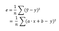
LSE calculates the least squares estimate:
least squaresbecause it takes the square of each error.errorbecausey' - yrepresents the difference between the estimated value and the real value. The square penalizes the error, the larger the difference is, the bigger the error will be.
Gradient descent
In order to find the best a and b which minimizes the cost function, we will apply Gradient descent.
In simple scenarios like this supermarket expenses, Gradient descent is very efficient. It allows us to converge toward a minima by using the derivatives of the cost function.
A derivative on a certain point of the function is the slope of the tangeant on that particular point.
Gradient is another word for slope.
This is the key of Gradient descent, it uses the slope to define its direction:
- When the slope is positive, the function is going upward therefore the minima is on the left
- When the slope is negative, the function is going downward therefore the minima is on the right
Using this two definitions, we can establish the following algorithm to converge to the minima (1):
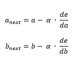
This is the core of Gradient descent, de/da and de/db are respectively the derivatives of the cost function in function of a and b.
On each step, we calculate the derivatives and update a and b.
With a bit of calculus, we can get de/da and de/db.
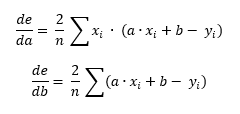
This is basically a g.f formula where (g.f)' = g'.f * f'.
a and b usually appear as theta1 and thetha0, so I will call them thetha1 and thetha0.
alpha is the learning rate. It represents the step to take between each iterations.
This constant is very important as it directly affects the results.
In order to find the alpha which suits your function, try to see how big are the derivatives and compensate with a smaller or bigger alpha to reduce the steps taken or increase it if too small.
So we will iterate over the algorithm to get the perfect thetha0 and thetha1.
When do we stop?
What worked for me was to set a definite number of iterations. Using a definite number is easy because you know how many iterations it will take to reach the result therefore you don’t risk to be stuck in an infinite loop. Obviously not all functions require the same number of iterations, but overall my supermarket expenses are “almost” the same every month therefore I could find a correct number of iterations.
Wonderful, you now know everything about the gradient descent!
3. Apply to real life data with FSharp
Before starting, we can already try to plot the cost function against thetha0 and thetha1 to get a better understanding of it.
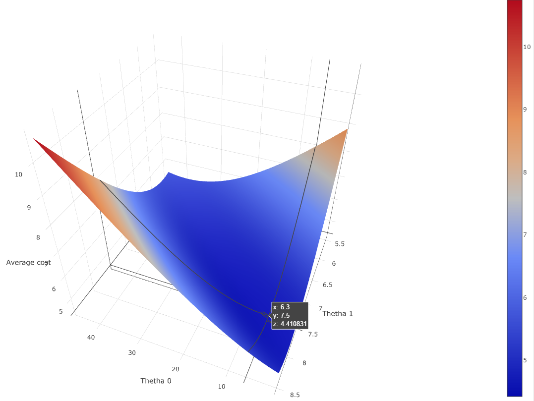
If you are confused by why the error range from 0 to 15, I squareroot-ed the the sum of squares of the error to get the average error.
Using this plot we can confirm that there is a mininma - around (6.3, 7.5) for an average cost error of 4.41 - therefore it should be feasible to program Gradient descent to converge to it.
Let’s start first by defining the settings of the Gradient descent.
type Settings = {
    LearningRate: float
    Dataset: List<float * float>
    Iterations: int
}
We have the learning rate alpha, the dataset a list of (x, y) and the number of iterations.
From #2, we learnt that to compute Gradient descent we only need to calculate thetha0 and thetha1 by iterating n time over the Gradient descent formula (1).
In the calculation of the thetha0 and thetha1, the only difference is the derivative calculation.
Even within the derivative calculation, the only difference is the inner derivative.
Knowing that we can define a generic function to calculate the next theta.
let nextThetha innerDerivative (settings: Settings) thetha =
    let sum =
        [0..settings.Dataset.Length - 1]
        |> List.map (fun i -> settings.Dataset.[i])
        |> List.map (fun (x, y) -> innerDerivative x y)
        |> List.sum

    thetha - settings.LearningRate * ((2./float settings.Dataset.Length) * sum)
Finally we can iterate n number of times and calculate the thetas.
let estimate settings =
    [0..settings.Iterations]
    |> List.scan (fun thethas _ ->
        match thethas with
        | thetha0::thetha1::_ ->

            let thetha0 =
                nextThetha (fun x y -> thetha0 + thetha1 * x - y) settings thetha0

            let thetha1 =
                nextThetha (fun x y -> (thetha0 + thetha1 * x - y) * x) settings thetha1

            [ thetha0; thetha1 ]

        | _ -> failwith "Could not compute next thethas, thethas are not in correct format.") [0.; 0.]
List.scan executes a fold and returns each iterations.
estimate will return the list of all thethas calculated on each iteration.
Using the results of each iterations we can plot the cost against each iteration.
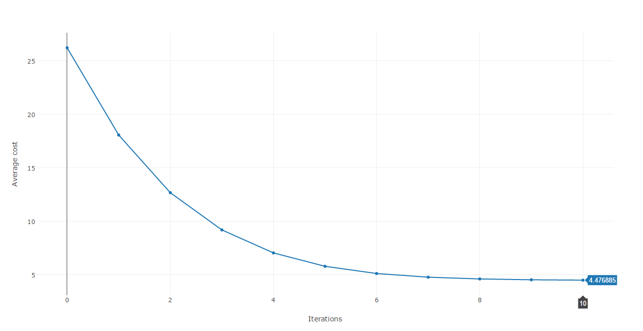
This cost function plot shows that we are heading to the right direction as after each iteration, the error is reduced dramatically until around the 8th iteration where it stabilizes at approximatively 4.45.
Lastely, in order to make this algorithm usable from everywhere, we create a model which will compute the correct thethas and return a function Estimate which will take a x and return an estimated y.
let createModel settings =
    let interationSteps = estimate settings

    match List.last interationSteps with
    | thetha0::thetha1::_ ->
        // returns a function which can be used to estimate y using the best thethas
        fun  x -> thetha0 + thetha1 * x

    | _ ->
        failwith "Failed to create model. Could not compute thethas."
By using the function returned by createModel, we can now visualize the best straight line which approximate the supermarket data.
Congratulation! You now know how Gradient descent work and you can now use it to minimize the cost function of a straight line which approximate supermarket expenses!
- Here the full
GradientDescentmodule can be found here https://github.com/Kimserey/DataExpenses/blob/master/London.Core/GradientDescent.fs. - The full test was coded from FSX and can be found here https://github.com/Kimserey/DataExpenses/blob/master/London/Gradient_Descent.fsx.
- The plots were produced using Plotly, the full index.html page can be found here https://github.com/Kimserey/DataExpenses/blob/master/London/index.html.
For convenience, here’s the full code of the GradientDecent module:
module GradientDescent =

    type Settings = {
        LearningRate: float
        Dataset: List<float * float>
        Iterations: int
    } with
        static member Default dataset = {
            LearningRate = 0.006
            Dataset = dataset
            Iterations = 5000
        }

    type ModelResult = {
        Estimate: float -> float
        Cost: Cost
        Thethas: float list
        ThethaCalculationSteps: ThethaCalculationSteps
    }

    and ThethaCalculationSteps = ThethaCalculationSteps of float list list
        with override x.ToString() = match x with ThethaCalculationSteps v -> sprintf "Thethas: %A" v

    and Cost = Cost of float
        with
            override x.ToString() = match x with Cost v -> sprintf "Cost: %.4f%%" v

            static member Value (Cost x) = x

            /// Computes the average cost
            static member Compute(data: List<float * float>, thethas: float list) =
                match thethas with
                | thetha0::thetha1::_ ->
                    let sum =
                        [0..data.Length - 1]
                        |> List.map (fun i -> data.[i])
                        |> List.map (fun (x, y) -> Math.Pow(thetha0 + thetha1 * x - y, 2.))
                        |> List.sum

                    Cost <| (1./float data.Length) * Math.Sqrt(sum)
                | _ -> failwith "Could not compute cost function, thethas are not in correct format."

    let nextThetha innerDerivative (settings: Settings) thetha =
        let sum =
            [0..settings.Dataset.Length - 1]
            |> List.map (fun i -> settings.Dataset.[i])
            |> List.map (fun (x, y) -> innerDerivative x y)
            |> List.sum

        thetha - settings.LearningRate * ((2./float settings.Dataset.Length) * sum)

    let estimate settings =
        [0..settings.Iterations - 1]
        |> List.scan (fun thethas _ ->
            match thethas with
            | thetha0::thetha1::_ ->
                let thetha0 = nextThetha (fun x y -> thetha0 + thetha1 * x - y) settings thetha0
                let thetha1 = nextThetha (fun x y -> (thetha0 + thetha1 * x - y) * x) settings thetha1
                [ thetha0; thetha1 ]
            | _ -> failwith "Could not compute next thethas, thethas are not in correct format.") [0.; 0.]

    let createModel settings =
        let interationSteps = estimate settings

        match List.last interationSteps with
        | thetha0::thetha1::_ as thethas->
            { Estimate = fun  x -> thetha0 + thetha1 * x
              Cost = Cost.Compute(settings.Dataset, thethas)
              Thethas = thethas
              ThethaCalculationSteps = ThethaCalculationSteps interationSteps }
        | _ -> failwith "Failed to create model. Could not compute thethas."
Conclusion
Today, we saw what Gradient descent was about.
What we did was to start from a problem which was to approximate a non-linear function representing supermarket expenses by reducing it to a linear function (straight line).
To do that, we used as the cost function the least squares estimate and programatically minimized it using Gradient descent.
We saw in details how to use Gradient descent to converge to a minima (or a maxima - by inversing the sign in the thetha iterations, we can converge to a maxima).
Gradient descent is a very simple algorithm, there are multiple variant and more complex things your can do with it but I wanted to show that it can be used simply for approximation like we did in this post.
Hope you enjoyed reading this post as much as I enjoyed writing it. As always if you have any comments, leave it here or hit me on Twitter https://twitter.com/Kimserey_Lam.
See you next time!
More posts you will like
If you like this post and are interested in manipulating dataframes, take a look at my other posts about Deedle - a data manipulation library, a piece of art to play with timeseries and dataframes.
- A primer on manipulating dataframe with Deedle: https://kimsereyblog.blogspot.co.uk/2016/04/a-primer-on-manipulating-data-frame.html
- Manipulating dataframe with Deedle Part 2: https://kimsereyblog.blogspot.co.uk/2016/06/manipulating-data-frame-with-deedle-in.html
Comments
Post a Comment